AFQ_example

Example AFQ analysis
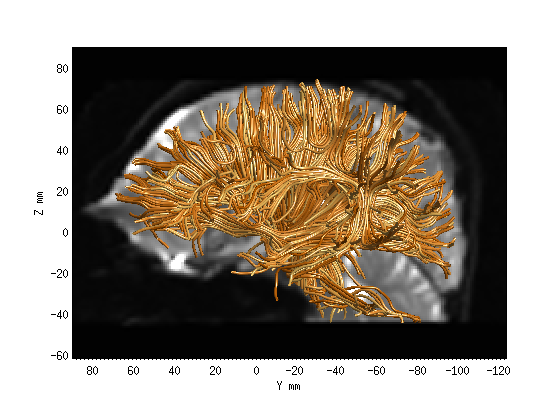
Step 1: Whole-brain tractography.
Step 2: Fiber tract segmentation
Step 3: Fiber tract cleaning
Step 4: Compute tract profiles
Step 5: Render Tract Profiles

Example AFQ analysis

% This will give an example of how to run each step in the AFQ pipeline for
% a single example subject's dataset that is included in the AFQ software.
% Once you add AFQ to your matlab search path you should be able to run all
% this code without any modifications.

Step 1: Whole-brain tractography.

% First we can use AFQ_directories to find the directories that contain the
% AFQ software and data on your local machine.
[AFQbase AFQdata AFQfunc AFQutil AFQdoc AFQgui] = AFQ_directories;

% The directory path to the first example subject within the AFQdata folder
% will be:
sub_dir = fullfile(AFQdata, 'control_01', 'dti30');

% Load the subject's dt6 file (generated from dtiInit).
dt = dtiLoadDt6(fullfile(sub_dir,'dt6.mat'));

% Track every fiber from a mask of white matter voxels. Use 'test' mode to
% track fewer fibers and make the example run quicker.
wholebrainFG = AFQ_WholebrainTractography(dt,'test');

% Visualize the wholebrain fiber group.  Because there are a few hundred
% thousand fibers we will use the 'numfibers' input to AFQ_RenderFibers to
% randomly select 1,000 fibers to render. The 'color' input is used to set
% the rgb values that specify the desired color of the fibers.
AFQ_RenderFibers(wholebrainFG, 'numfibers',1000, 'color', [1 .6 .2]);

% Add a sagittal slice from the subject's b0 image to the plot. First load
% the b0 image.
b0 = readFileNifti(fullfile(sub_dir,'bin','b0.nii.gz'));

% Then add the slice X = -2 to the 3d rendering.
AFQ_AddImageTo3dPlot(b0,[-2, 0, 0]);

scale=[2.0,2.0,2.0]mm, track=1, interp=1, step=1.0mm, fa=0.20, angle=30.0deg, puncture=0.20, minLength=50.0mm, maxLength=250.0mm
Tracking 33670 fibers (421 fibers per tick):
................................................................................
19833 fibers passed length threshold of 50.0 (out of 33670 seeds).
Elapsed time is 26.902815 seconds.
19833 fibers, mean length 97mm (max 251mm; min 50mm).

mesh can be rotated with arrow keys

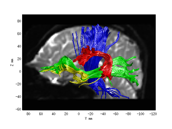
Step 2: Fiber tract segmentation

% Segment the whole-brain fiber group into 20 fiber tracts
fg_classified = AFQ_SegmentFiberGroups(dt, wholebrainFG);

% fg_classified.subgroup defines the fascicle that each fiber belongs to.
% We can convert fg_classified to a 1x20 structured array of fiber groups
% where each entry in the array is a segmented fiber tract. For example
% fg_classified(3) is the left corticospinal tract, fg_classified(11) is
% the left inferior fronto-occipital fasciculus (IFOF), fg_classified(17)
% is the left uncinate fasiculus,  and fg_classified(19) is the left
% arcuate fasciculus.
fg_classified = fg2Array(fg_classified);

% Render 400 corticospinal tract fibers in blue.
AFQ_RenderFibers(fg_classified(3),'numfibers',400,'color',[0 0 1]);

% Render 400 IFOF fibers in green. To add this tract to the same
% plotting window set the 'newfig' input to false.
AFQ_RenderFibers(fg_classified(11),'numfibers',400,'color',[0 1 0],'newfig',false)

% Render 400 uncinate fibers in yellow
AFQ_RenderFibers(fg_classified(17),'numfibers',400,'color',[1 1 0],'newfig',false)

% Render 400 arcuate fibers in green.
AFQ_RenderFibers(fg_classified(19),'numfibers',400,'color',[1 0 0],'newfig',false)

% Then add the slice X = -2 to the 3d rendering.
AFQ_AddImageTo3dPlot(b0,[-2, 0, 0]);

You chose to recompute ROIs
Fibers that get as close to the ROIs as 2mm will become candidates for the Mori Groups
Smoothing by 0 & 8mm..
Coarse Affine Registration..
Fine Affine Registration..
3D CT Norm...
 iteration  1:  FWHM =  13.31 Var = 24.3369
 iteration  2:  FWHM =  10.26 Var = 2.3268
 iteration  3:  FWHM =    9.9 Var = 1.82368
 iteration  4:  FWHM =  9.811 Var = 1.68895
 iteration  5:  FWHM =  9.746 Var = 1.62451
 iteration  6:  FWHM =  9.729 Var = 1.60517
 iteration  7:  FWHM =  9.714 Var = 1.59288
 iteration  8:  FWHM =  9.708 Var = 1.5878
 iteration  9:  FWHM =    9.7 Var = 1.58208
 iteration 10:  FWHM =  9.701 Var = 1.58178
 iteration 11:  FWHM =  9.698 Var = 1.58025
 iteration 12:  FWHM =  9.698 Var = 1.57987
 iteration 13:  FWHM =  9.697 Var = 1.57926
 iteration 14:  FWHM =  9.697 Var = 1.57926
 iteration 15:  FWHM =  9.696 Var = 1.57881
 iteration 16:  FWHM =  9.697 Var = 1.57881
Computing inverse deformation...
dtiCleanFibers: Keeping 19727 out of 19833 fibers.
dtiSplitInterhemisphericFibers: Splitting every fiber below Z=-10 

mesh can be rotated with arrow keys

ans =

     []


ans =

     []


ans =

     []

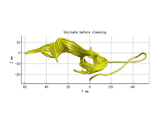
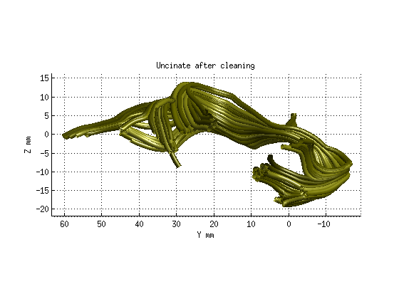
Step 3: Fiber tract cleaning

% Even though the fiber tracts produced by AFQ_SegementFiberGroups conform
% to the cannonical definition of the of each tract, there are still some
% abherrant fibers that deviate from the core of the fascicle. For example
% notice for the uncinate a few fibers deviate from the typical trajectory
% and take a weird loop. AFQ_removeFiberOutliers can be used to identify
% and remove abherrant fibers.

% Create a new variable for the left uncinate
uf = fg_classified(17);
% Remove fibers more than maxDist standard deviations from the tract core
maxDist = 4;
% Remove fibers more than maxLen standard deviations above the mean length
maxLen = 4;
% Sample each fiber to numNodes points
numNodes = 30;
% Compute the tract core with the function M
M = 'mean';
% Maximum number of iterations
maxIter = 1;
% Display the number of fibers removed in each iteration
count = true;

% Begin cleaning the uncinate
uf_clean = AFQ_removeFiberOutliers(uf,maxDist,maxLen,numNodes,M,count,maxIter);

% Notice that the final fiber group is much cleaner than the origional.
% There are not as many long looping fibers that deviate from the fascicle.
AFQ_RenderFibers(uf,'numfibers',1000,'color',[1 1 0]);
title('Uncinate before cleaning','fontsize',18)
AFQ_RenderFibers(uf_clean,'numfibers',1000,'color',[.5 .5 0]);
title('Uncinate after cleaning','fontsize',18)

% Loop over all 20 fiber groups and clean each one
for ii = 1:20
    fg_clean(ii) = AFQ_removeFiberOutliers(fg_classified(ii),maxDist,maxLen,numNodes,M,count,maxIter);
end

Left Uncinate number of fibers: 110 
Left Uncinate number of fibers: 106 
mesh can be rotated with arrow keys

mesh can be rotated with arrow keys

Left Thalamic Radiation number of fibers: 260 
Left Thalamic Radiation number of fibers: 234 
Right Thalamic Radiation number of fibers: 220 
Right Thalamic Radiation number of fibers: 202 
Left Corticospinal number of fibers: 828 
Left Corticospinal number of fibers: 777 
Right Corticospinal number of fibers: 1031 
Right Corticospinal number of fibers: 1009 
Left Cingulum Cingulate number of fibers: 97 
Left Cingulum Cingulate number of fibers: 86 
Right Cingulum Cingulate number of fibers: 14 
Left Cingulum Hippocampus number of fibers: 29 
Left Cingulum Hippocampus number of fibers: 28 
Right Cingulum Hippocampus number of fibers: 23 
Right Cingulum Hippocampus number of fibers: 21 
Callosum Forceps Major number of fibers: 262 
Callosum Forceps Major number of fibers: 251 
Callosum Forceps Minor number of fibers: 942 
Callosum Forceps Minor number of fibers: 925 
Left IFOF number of fibers: 300 
Left IFOF number of fibers: 273 
Right IFOF number of fibers: 165 
Right IFOF number of fibers: 155 
Left ILF number of fibers: 106 
Left ILF number of fibers: 101 
Right ILF number of fibers: 151 
Right ILF number of fibers: 136 
Left SLF number of fibers: 115 
Left SLF number of fibers: 108 
Right SLF number of fibers: 282 
Right SLF number of fibers: 272 
Left Uncinate number of fibers: 110 
Left Uncinate number of fibers: 106 
Right Uncinate number of fibers: 251 
Right Uncinate number of fibers: 238 
Left Arcuate number of fibers: 262 
Left Arcuate number of fibers: 241 
Right Arcuate number of fibers: 99 
Right Arcuate number of fibers: 90

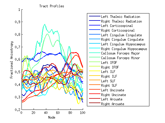
Step 4: Compute tract profiles

% AFQ_ComputeTractProperties will compute diffusion properties (FA, MD, RD,
% AD, etc.) at numNodes locations along the trajectory of each fiber tract.
% The default of the function is to do this computation for the portion of
% the tract spanning between the two defining ROIs.
numNodes = 100;
[fa md rd ad] = AFQ_ComputeTractProperties(fg_clean, dt, numNodes);

% Open a new figure window
figure; hold('on');
% Set the coloring of each plot
set(gca,'ColorOrder',jet(20));
% Plot the Tract FA Profiles for each tract
plot(fa,'linewidth',2);
xlabel('Node');
ylabel('Fractional Anisotropy');
title('Tract Profiles');
% Add a legend with the names of each fiber tract. Here are the names of
% each fiber group.
fgNames={'Left Thalmic Radiation','Right Thalmic Radiation'...
    'Left Corticospinal','Right Corticospinal', 'Left Cingulum Cingulate'...
    'Right Cingulum Cingulate', 'Left Cingulum Hippocampus'...
    'Right Cingulum Hippocampus', 'Callosum Forceps Major'...
    'Callosum Forceps Minor', 'Left IFOF','Right IFOF','Left ILF'...
    'Right ILF','Left SLF','Right SLF','Left Uncinate','Right Uncinate'...
    'Left Arcuate','Right Arcuate'};
legend(fgNames,'Location','EastOutside' );

Step 5: Render Tract Profiles

% Render the Tract FA Profile for the left arcuate fasciculus. When the
% argument 'dt' is passed in follwed by a variable containing the dt6
% structure then the tract profile is added to the plot. The colormap
% denotes the FA value at each point along the tract core.
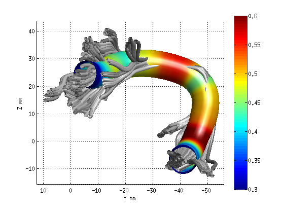
AFQ_RenderFibers(fg_clean(19),'dt',dt);

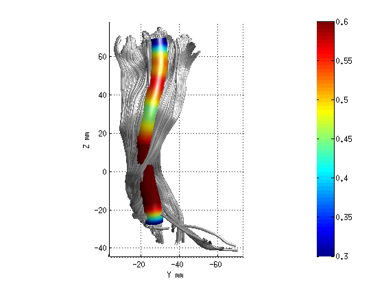
% Render the Tract FA Profile for the left corticospinal tract
AFQ_RenderFibers(fg_clean(3),'dt',dt);

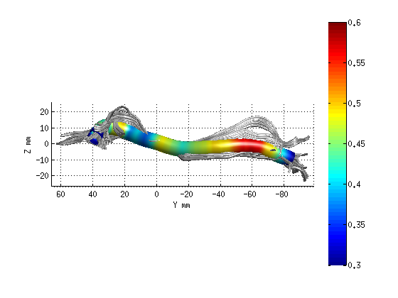
% Render the Tract FA Profile for the left IFOF
AFQ_RenderFibers(fg_clean(11),'dt',dt);

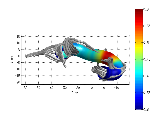
% Render the Tract FA Profile for the left uncinate
AFQ_RenderFibers(fg_clean(17),'dt',dt);

mesh can be rotated with arrow keys

mesh can be rotated with arrow keys

mesh can be rotated with arrow keys

mesh can be rotated with arrow keys

Contents

Example AFQ analysis

Step 1: Whole-brain tractography.

Step 2: Fiber tract segmentation

Step 3: Fiber tract cleaning

Step 4: Compute tract profiles

Step 5: Render Tract Profiles