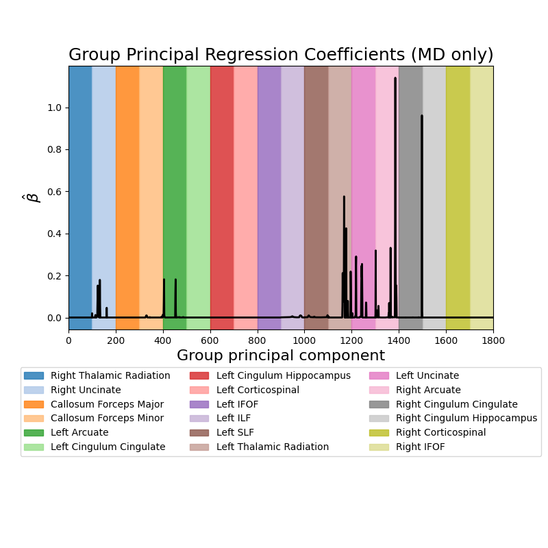
Predict age from white matter features

Predict subject age from white matter features. This example fetches the Weston-Havens dataset described in Yeatman et al 1. This dataset contains tractometry features from 77 subjects ages 6-50. The plots display the absolute value of the mean regression coefficients (averaged across cross-validation splits) for the mean diffusivity (MD) features.

Predictive performance for this example is quite poor. In a research setting, one might have to ensemble a number of SGL estimators together and conduct a more thorough search of the hyperparameter space. For more details, please see 2.

1

Jason D. Yeatman, Brian A. Wandell, & Aviv A. Mezer, “Lifespan maturation and degeneration of human brain white matter” Nature Communications, vol. 5:1, pp. 4932, 2014 DOI: 10.1038/ncomms5932

2

Adam Richie-Halford, Jason Yeatman, Noah Simon, and Ariel Rokem “Multidimensional analysis and detection of informative features in human brain white matter” PLOS Computational Biology, 2021 DOI: 10.1371/journal.pcbi.1009136

import matplotlib.pyplot as plt
import numpy as np
import os.path as op

from afqinsight.datasets import download_weston_havens, load_afq_data
from afqinsight import make_afq_regressor_pipeline

from sklearn.model_selection import cross_validate

Fetch example data

The download_weston_havens() function download the data used in this example and places it in the ~/.cache/afq-insight/weston_havens directory. If the directory does not exist, it is created. The data follows the format expected by the load_afq_data() function: a file called nodes.csv that contains AFQ tract profiles and a file called subjects.csv that contains information about the subjects. The two files are linked through the subjectID column that should exist in both of them. For more information about this format, see also the AFQ-Browser documentation (items 2 and 3).

workdir = download_weston_havens()

Downloading https://yeatmanlab.github.io/AFQBrowser-demo/data/nodes.csv to ../../../../.cache/afq-insight/weston_havens_data/nodes.csv.
Downloading https://yeatmanlab.github.io/AFQBrowser-demo/data/subjects.csv to ../../../../.cache/afq-insight/weston_havens_data/subjects.csv.

Read in the data

Next, we read in the data. The load_afq_data() function expects a string input that points to a directory that holds appropriately-shaped data and returns variables that we will use below in our analysis of the data.

afqdata = load_afq_data(
    fn_nodes=op.join(workdir, "nodes.csv"),
    fn_subjects=op.join(workdir, "subjects.csv"),
    dwi_metrics=["md", "fa"],
    target_cols=["Age"],
)

# afqdata is a namedtuple. You can access it's fields using dot notation or by
# unpacking the tuple. To see all of the available fields use `afqdata._fields`
X = afqdata.X
y = afqdata.y
groups = afqdata.groups
feature_names = afqdata.feature_names
group_names = afqdata.group_names
subjects = afqdata.subjects

Create an analysis pipeline

pipe = make_afq_regressor_pipeline(
    imputer_kwargs={"strategy": "median"},  # Use median imputation
    use_cv_estimator=True,  # Automatically determine the best hyperparameters
    scaler="standard",  # Standard scale the features before regression
    groups=groups,
    verbose=0,  # Be quiet!
    pipeline_verbosity=False,  # No really, be quiet!
    tuning_strategy="bayes",  # Use BayesSearchCV to determine the optimal hyperparameters
    n_bayes_iter=10,  # Consider only this many points in hyperparameter space
    cv=3,  # Use three CV splits to evaluate each hyperparameter combination
    l1_ratio=[0.0, 1.0],  # Explore the entire range of ``l1_ratio``
    eps=5e-2,  # This is the ratio of the smallest to largest ``alpha`` value
    tol=1e-2,  # Set a lenient convergence tolerance just for this example
)

# ``pipe`` is a scikit-learn pipeline and can be used in other scikit-learn
# functions. For example, here we are doing 5-fold cross-validation using scikit
# learn's :func:`cross_validate` function.

scores = cross_validate(
    pipe, X, y, cv=5, return_train_score=True, return_estimator=True
)

print(f"Mean train score: {np.mean(scores['train_score']):5.3f}")
print(f"Mean test score:  {np.mean(scores['test_score']):5.3f}")
print(f"Mean fit time:    {np.mean(scores['fit_time']):5.2f}s")
print(f"Mean score time:  {np.mean(scores['score_time']):5.2f}s")

mean_coefs = np.mean(
    np.abs([est.named_steps["estimate"].coef_ for est in scores["estimator"]]), axis=0
)

fig, ax = plt.subplots(1, 1, figsize=(8, 8))
_ = ax.plot(mean_coefs[1800:], color="black", lw=2)
_ = ax.set_xlim(0, 1800)

colors = plt.get_cmap("tab20").colors
for grp, grp_name, color in zip(groups[:18], group_names[18:], colors):
    _ = ax.axvspan(grp.min(), grp.max() + 1, color=color, alpha=0.8, label=grp_name[1])

box = ax.get_position()
ax.set_position([box.x0, box.y0 + box.height * 0.375, box.width, box.height * 0.625])

_ = ax.legend(loc="upper center", bbox_to_anchor=(0.5, -0.125), ncol=3)
_ = ax.set_ylabel(r"$\hat{\beta}$", fontsize=16)
_ = ax.set_xlabel("Group principal component", fontsize=16)
_ = ax.set_title("Group Principal Regression Coefficients (MD only)", fontsize=18)

Mean train score: 0.906
Mean test score:  -0.373
Mean fit time:    14.73s
Mean score time:   0.00s