Classify ALS diagnosis from white matter features

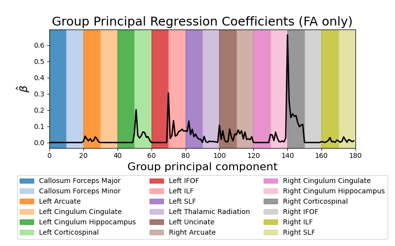
Predict ALS diagnosis from white matter features. This example fetches the ALS classification dataset from Sarica et al 1. This dataset contains tractometry features from 24 patients with ALS and 24 demographically matched control subjects. The plots display the absolute value of the mean regression coefficients (averaged across cross-validation splits) for the fractional anisotropy (FA) features.

To save computational time, we take the first 10 principal components from each feature group (i.e. from each metric-bundle combination). For more details on this approach in a research setting, please see 2.

1

Alessia Sarica, et al. “The Corticospinal Tract Profile in AmyotrophicLateral Sclerosis” Human Brain Mapping, vol. 38, pp. 727-739, 2017 DOI: 10.1002/hbm.23412

2

Adam Richie-Halford, Jason Yeatman, Noah Simon, and Ariel Rokem “Multidimensional analysis and detection of informative features in human brain white matter” PLOS Computational Biology, 2021 DOI: 10.1371/journal.pcbi.1009136

Downloading https://github.com/yeatmanlab/Sarica_2017/raw/gh-pages/data/nodes.csv to ../../../../.cache/afq-insight/sarica_data/nodes.csv.
Downloading https://github.com/yeatmanlab/Sarica_2017/raw/gh-pages/data/subjects.csv to ../../../../.cache/afq-insight/sarica_data/subjects.csv.
Mean train score: 1.000
Mean test score:  0.751
Mean fit time:    10.52s
Mean score time:   0.01s

import matplotlib.pyplot as plt
import numpy as np
import os.path as op

from afqinsight.datasets import download_sarica, load_afq_data
from afqinsight import make_afq_classifier_pipeline

from groupyr.decomposition import GroupPCA

from sklearn.impute import SimpleImputer
from sklearn.model_selection import cross_validate

workdir = download_sarica()

afqdata = load_afq_data(
    fn_nodes=op.join(workdir, "nodes.csv"),
    fn_subjects=op.join(workdir, "subjects.csv"),
    dwi_metrics=["md", "fa"],
    target_cols=["class"],
    label_encode_cols=["class"],
)

# afqdata is a namedtuple. You can access it's fields using dot notation or by
# unpacking the tuple. To see all of the available fields use `afqdata._fields`
X = afqdata.X
y = afqdata.y
groups = afqdata.groups
feature_names = afqdata.feature_names
group_names = afqdata.group_names
subjects = afqdata.subjects

# Here we reduce computation time by taking the first 10 principal components of each feature group and performing SGL logistic regression on those components.
# If you want to train an SGL model without group PCA, set ``do_group_pca = False``. This will increase the number of features by an order of magnitude and slow down execution time.
do_group_pca = True

if do_group_pca:
    n_components = 10

    # The next three lines retrieve the group structure of the group-wise PCA
    # and store it in ``groups_pca``. We do not use the imputer or GroupPCA transformer
    # for anything else
    imputer = SimpleImputer(strategy="median")
    gpca = GroupPCA(n_components=n_components, groups=groups)
    groups_pca = gpca.fit(imputer.fit_transform(X)).groups_out_

    transformer = GroupPCA
    transformer_kwargs = {"groups": groups, "n_components": n_components}
else:
    transformer = False
    transformer_kwargs = None

pipe = make_afq_classifier_pipeline(
    imputer_kwargs={"strategy": "median"},  # Use median imputation
    use_cv_estimator=True,  # Automatically determine the best hyperparameters
    feature_transformer=transformer,  # See note above about group PCA
    feature_transformer_kwargs=transformer_kwargs,
    scaler="standard",  # Standard scale the features before regression
    groups=groups_pca
    if do_group_pca
    else groups,  # SGL will use the original feature groups or the PCA feature groups depending on the choice above
    verbose=0,  # Be quiet!
    pipeline_verbosity=False,  # No really, be quiet!
    tuning_strategy="bayes",  # Use BayesSearchCV to determine the optimal hyperparameters
    n_bayes_iter=20,  # Consider only this many points in hyperparameter space
    cv=3,  # Use three CV splits to evaluate each hyperparameter combination
    l1_ratio=[0.0, 1.0],  # Explore the entire range of ``l1_ratio``
    eps=5e-2,  # This is the ratio of the smallest to largest ``alpha`` value
    tol=1e-2,  # Set a lenient convergence tolerance just for this example
)

# ``pipe`` is a scikit-learn pipeline and can be used in other scikit-learn functions
scores = cross_validate(
    pipe, X, y, cv=5, return_train_score=True, return_estimator=True
)

print(f"Mean train score: {np.mean(scores['train_score']):5.3f}")
print(f"Mean test score:  {np.mean(scores['test_score']):5.3f}")
print(f"Mean fit time:    {np.mean(scores['fit_time']):5.2f}s")
print(f"Mean score time:  {np.mean(scores['score_time']):5.2f}s")

mean_coefs = np.mean(
    np.abs([est.named_steps["estimate"].coef_ for est in scores["estimator"]]), axis=0
)

fig, ax = plt.subplots(1, 1, figsize=(8, 5))
_ = ax.plot(mean_coefs[:180], color="black", lw=2)
_ = ax.set_xlim(0, 180)

colors = plt.get_cmap("tab20").colors
for grp, grp_name, color in zip(groups_pca[:18], group_names, colors):
    _ = ax.axvspan(grp.min(), grp.max() + 1, color=color, alpha=0.8, label=grp_name[1])

box = ax.get_position()
_ = ax.set_position(
    [box.x0, box.y0 + box.height * 0.375, box.width, box.height * 0.625]
)

_ = ax.legend(loc="upper center", bbox_to_anchor=(0.5, -0.2), ncol=3)
_ = ax.set_ylabel(r"$\hat{\beta}$", fontsize=16)
_ = ax.set_xlabel("Group principal component", fontsize=16)
_ = ax.set_title("Group Principal Regression Coefficients (FA only)", fontsize=18)