Note
Go to the end to download the full example code.
Getting started programming with pyAFQ#
There are two ways to use pyAFQ: through the command line interface, and by writing Python code. This tutorial will walk you through the basics of the latter, using pyAFQ’s Python Application Programming Interface (API).
import os.path as op
import matplotlib.pyplot as plt
import nibabel as nib
import plotly
import pandas as pd
from AFQ.api.group import GroupAFQ
import AFQ.data.fetch as afd
import AFQ.viz.altair as ava
Example data#
pyAFQ assumes that the data is organized in a BIDS compliant directory. To get users started with this tutorial, we will download some example data and organize it in a BIDS compliant way (for more details on how BIDS is used in pyAFQ, refer to bids_tutorial).
The following call dowloads a dataset that contains a single subject’s high angular resolution diffusion imaging (HARDI) data, collected at the Stanford Vista Lab
Note
See https://purl.stanford.edu/ng782rw8378 for details on dataset.
The data are downloaded and organized locally into a BIDS compliant
anatomical data folder (anat) and a diffusion-weighted imaging data
(dwi) folder, which are both placed in the user’s home directory under:
``~/AFQ_data/stanford_hardi/``
The data is also placed in a derivatives directory, signifying that it has already undergone the required preprocessing necessary for pyAFQ to run.
The clear_previous_afq is used to remove any previous runs of the afq object stored in the ~/AFQ_data/stanford_hardi/ BIDS directory. Set it to None if you want to use the results of previous runs.
afd.organize_stanford_data(clear_previous_afq="track")
Set tractography parameters (optional)#
We make create a tracking_params variable, which we will pass to the
GroupAFQ object which specifies that we want 25,000 seeds randomly
distributed in the white matter. We only do this to make this example
faster and consume less space. We also set num_chunks to True,
which will use ray to parallelize the tracking across all cores.
This can be removed to process in serial, or set to use a particular
distribution of work by setting n_chunks to an integer number.
tracking_params = dict(n_seeds=25000,
random_seeds=True,
rng_seed=2022,
trx=True,
num_chunks=True)
Initialize a GroupAFQ object:#
Creates a GroupAFQ object, that encapsulates tractometry. This object can be used to manage the entire AFQ pipeline, including:
Tractography
Registration
Segmentation
Cleaning
Profiling
Visualization
This will also create an output folder for the corresponding AFQ derivatives
in the AFQ data directory: AFQ_data/stanford_hardi/derivatives/afq/
To initialize this object we will pass in the path location to our BIDS compliant data, the name of the preprocessing pipeline we want to use, and the tracking parameters we defined above. We will also specify the visualization backend we want to use (see below for more details). We will also be using plotly to generate an interactive visualization. The value plotly_no_gif indicates that interactive visualizations will be generated as html web-pages that can be opened in a browser, but not as static gif files.
myafq = GroupAFQ(
bids_path=op.join(afd.afq_home, 'stanford_hardi'),
preproc_pipeline='vistasoft',
tracking_params=tracking_params,
viz_backend_spec='plotly_no_gif')
Calculating DTI FA (Diffusion Tensor Imaging Fractional Anisotropy)#
The GroupAFQ object has a method called export, which allows the user to calculate various derived quantities from the data.
For example, FA can be computed using the DTI model, by explicitly calling myafq.export(“dti_fa”). This triggers the computation of DTI parameters for all subjects in the dataset, and stores the results in the AFQ derivatives directory. In addition, it calculates the FA from these parameters and stores it in a different file in the same directory.
Note
The AFQ API computes quantities lazily. This means that DTI parameters are not computed until they are required. This means that the first line below is the one that requires time.
The result of the call to export is a dictionary, with the subject IDs as keys, and the filenames of the corresponding files as values. This means that to extract the filename corresponding to the FA of the first subject, we can do:
Visualize the result with Matplotlib#
At this point FA is an array, and we can use standard Python tools to visualize it or perform additional computations with it.
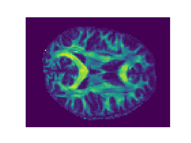
In this case we are going to take an axial slice halfway through the FA data array and plot using a sequential color map.
Note
The data array is structured as a xyz coordinate system.

(-0.5, 105.5, 80.5, -0.5)
Recognizing the bundles and calculating act profiles:#
Typically, users of pyAFQ are interested in calculating not only an overall map of the FA, but also the major white matter pathways (or bundles) and tract profiles of tissue properties along their length. To trigger the pyAFQ pipeline that calculates the profiles, users can call the export(‘profiles’) method:
Note
Running the code below triggers the full pipeline of operations leading to the computation of the tract profiles. Therefore, it takes a little while to run (about 40 minutes, typically).
myafq.export('profiles')
(TractActor pid=5267)
0it [00:00, ?it/s]
(TractActor pid=5267)
1it [00:01, 1.38s/it]
(TractActor pid=5274)
0it [00:00, ?it/s] [repeated 2x across cluster] (Ray deduplicates logs by default. Set RAY_DEDUP_LOGS=0 to disable log deduplication, or see https://docs.ray.io/en/master/ray-observability/user-guides/configure-logging.html#log-deduplication for more options.)
(TractActor pid=5267)
1062it [00:06, 216.95it/s] [repeated 135x across cluster]
(TractActor pid=5267)
2146it [00:11, 213.05it/s] [repeated 138x across cluster]
(TractActor pid=5267)
3196it [00:16, 209.44it/s] [repeated 137x across cluster]
(TractActor pid=5267)
4241it [00:21, 182.54it/s] [repeated 136x across cluster]
(TractActor pid=5266)
4228it [00:25, 152.05it/s] [repeated 135x across cluster]
(TractActor pid=5266)
5086it [00:30, 164.50it/s] [repeated 137x across cluster]
{'01': '/home/runner/AFQ_data/stanford_hardi/derivatives/afq/sub-01/ses-01/sub-01_ses-01_coordsys-RASMM_trkmethod-probCSD_recogmethod-AFQ_desc-profiles_dwi.csv'}
Visualizing the bundles and calculating act profiles:#
The pyAFQ API provides several ways to visualize bundles and profiles.
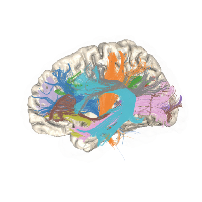
First, we will run a function that exports an html file that contains an interactive visualization of the bundles that are segmented.
Note
By default we resample a 100 points within a bundle, however to reduce processing time we will only resample 50 points.
Once it is done running, it should pop a browser window open and let you interact with the bundles.
Note
You can hide or show a bundle by clicking the legend, or select a single bundle by double clicking the legend. The interactive visualization will also all you to pan, zoom, and rotate.
bundle_html = myafq.export("all_bundles_figure")
plotly.io.show(bundle_html["01"][0])
